0%

用python从零实现一个神经网络

不用tensorflow、pytorch等任何现有深度学习框架以及各种封装好的机器学习库,仅使用python语言及矩阵运算的库,从零开始实现一个全联接的神经网络。

任务描述

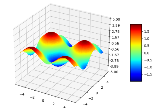
我们以一个回归任务为例,实现一个多层神经网络来拟合一个非线性函数$ y= \sin (x_{1})- \cos (x_{2}),x_{1} \in \left[ -5,5 \right] ,x_{2} \in \left[ -5,5 \right] $,函数图像如下图所示,输入层包含2个神经元,输出层包含1个神经元,隐藏层的数目和神经元数自定义,隐藏层采用ReLU作为激活函数,输出层用恒等函数做为激活函数,损失函数为均方误差(MSE)。

实际上我们实现的神经网络可以自定义输入输出大小、隐藏层结构、激活函数、损失函数等,因此用在其他任务上也是完全可以的。

1

准备工作

训练神经网络之前,我们需要先完成一些准备工作,包括生成训练和验证的数据集、定义用到的激活函数和损失函数。

数据集生成

在轴$x_1$和$x_2$的$[-5,5]$区间上每隔0.1均匀地对样本点进行采样,然后计算目标函数的值,生成100*100=10000个训练数据,转换成为numpy​矩阵,作为训练数据集:

1
2
3
4
5
6
7
8
9
# 生成训练数据集
x_train = []
y_train = []
for x1 in np.arange(-5, 5, 0.1):
for x2 in np.arange(-5, 5, 0.1):
x_train.append([x1, x2])
y_train.append(np.sin(x1)-np.cos(x2))
x_train = np.array(x_train)
y_train = np.array(y_train)

另外随机采样并生成大小为1000的验证数据集:

1
2
3
4
5
6
7
8
9
10
11
# 生成验证数据集
x_val = []
y_val = []
for i in range(1000):
x1 = random.uniform(-5, 5)
x2 = random.uniform(-5, 5)
x_val.append([x1, x2])
y_val.append(np.sin(x1)-np.cos(x2))
x_val = np.array(x_val)
y_val = np.array(y_val)

激活函数和损失函数

定义本次任务用到的数学函数,包括激活函数和损失函数:

  • 激活函数

    定义ActivationFunction类作为激活函数的基类,包括calculate(计算)和derivative(求导)两个抽象方法。本次任务中用到了ReLU和Pureline两种激活函数,若想使用其他激活函数可以仿照下面的形式定义(注意接受的参数x都是一个numpy矩阵)。

    1
    2
    3
    4
    5
    6
    7
    8
    9
    10
    11
    12
    13
    14
    15
    16
    17
    18
    19
    20
    21
    22
    23
    24
    25
    26
    27
    28
    29
    30
    31
    32
    33
    34
    35
    36
    import numpy as np
    from abc import ABCMeta, abstractmethod

    class ActivationFunction:
    '''激活函数基类'''
    __metaclass__ = ABCMeta

    @abstractmethod
    def calculate(self, x):
    pass

    @abstractmethod
    def derivative(self, x):
    pass

    class ReLU(ActivationFunction):
    '''relu激活函数'''

    @classmethod
    def calculate(self, x):
    return np.maximum(x, 0)

    @classmethod
    def derivative(self, x):
    return np.where(x > 0, 1, 0)

    class Pureline(ActivationFunction):
    '''恒等激活函数'''

    @classmethod
    def calculate(self, x):
    return x

    @classmethod
    def derivative(self, x):
    return np.ones(shape=x.shape)
  • MSE损失函数

    假设样本个数为$n$,计算公式:$MSE=\frac{1}{n} \sum_{i=1}^{n}(y_{true}[i]-y_{pred}[i])^2$

    1
    2
    3
    def mse_loss(y_true, y_pred):
    '''MSE损失函数'''
    return ((y_true - y_pred) ** 2).mean()

模型训练

数据结构定义和初始化

首先定义类NeuralNetwork表示神经网络类,初始化时用户向类构造函数传入参数input_size(输入层维度)、output_size(输出层维度)、hidden_size(隐藏层维度,用一个数组表示,如[5,3]表示两个隐藏层,分别包含5个和3个神经元),从而可以达到任意调整神经网络结构的目的。

接着定义两个数组self.w和self.b表示神经网络的权重和偏移量,每层的权重是一个numpy矩阵,用np.random.normal函数进行高斯分布初始化(设置均值为0,方差为0.1);同时定义一个数组self.activations表示每层的激活函数,这里隐藏层激活函数为ReLU,输出层激活函数为Pureline:

1
2
3
4
5
6
7
8
9
10
11
12
13
14
15
16
# 随机初始化权重和偏移量
self.len = len(hidden_size) + 1 # 层数(除输入层)
loc = 0.0
scale = 0.1
# 隐藏层
self.w = [np.random.normal(loc, scale, size=(input_size, hidden_size[0]))]
self.b = [np.random.normal(loc, scale, size=(hidden_size[0],))]
self.activations = [ReLU]
for i in range(len(hidden_size)-1):
self.w.append(np.random.normal(loc, scale, size=(hidden_size[i], hidden_size[i+1])))
self.b.append(np.random.normal(loc, scale, size=(hidden_size[i+1],)))
self.activations.append(ReLU)
# 输出层
self.w.append(np.random.normal(loc, scale, size=(hidden_size[-1], output_size)))
self.b.append(np.random.normal(loc, scale, size=(output_size,)))
self.activations.append(Pureline)

然后定义五个数组用于保存训练时的中间结果,均初始化为全0:

  • self.z:每个神经元激活前的输出。
  • self.a:每个神经元激活后的输出。
  • self.delta:神经单元误差$\delta$,即loss对每个神经元激活前输出$z$的梯度(用于反向传播更新权重)。
  • self.delta_w:权重w的累积更新值,用于处理完每个batch后更新权重。
  • self.delta_b:权重b的累积更新值。

前向计算中间结果

每轮训练首先调用一个自定义的shuffle方法打乱训练样本集合。然后开始训练,设置训练轮数为30,batch_size为10,初始学习率为0.01。对每个输入样本,通过前向传播计算得到每层的输出self.z和self.a,如假设第$i$层($i>1$)的输入为$a[i-1]$,权重和偏移为$w[i]$和$b[i]$,则有:

$z[i]=a[i-1]\times w[i] + b[i]$,

$a[i]=activations[i].calculate(z[i])$

1
2
3
4
5
6
7
8
9
10
11
12
13
14
15
16
17
18
19
20
21
22
23
def shuffle(x, y):
'''随机打乱数据'''
xy= np.c_[x,y]
np.random.shuffle(xy)
x = xy[:, :-1]
y = xy[:, -1]
return x, y

def train(self, x_train, y_train, x_val, y_val, epochs=30, batch_size=10, lr=0.01):
'''训练模型'''

self.validate(0, x_train, y_train, x_val, y_val)

for epoch in range(epochs):
x_train_shuffle, y_train_shuffle = shuffle(x_train, y_train)
batch_count = 0
for x, y_true in zip(x_train_shuffle, y_train_shuffle):
# 前向传播得到每层输出
layer_output = x
for layer in range(0, self.len):
self.z[layer] = np.matmul(layer_output, self.w[layer]) + self.b[layer]
layer_output = self.activations[layer].calculate(self.z[layer])
self.a[layer] = layer_output

反向传播计算梯度

接下来计算输出层(第-1层)的神经单元误差$\delta$,对于每个样本,假如输出层维度为$m$,损失函数$C=\frac{1}{m}\sum_{i=1}^{m}(y_{true}[i]-a[-1][i])^2$(本次任务中$m=1$),则$\delta[-1] = \frac{\partial C}{\partial z[-1]} = \frac{\partial C}{\partial a[-1]} \cdot \frac{\partial a[-1]}{\partial z[-1]}= \frac{1}{m} \cdot 2 \cdot (a[-1] - y_{true}) \cdot \theta’(z[-1])$,其中$\theta$为输出层的激活函数。

然后可以通过递推式反向计算出前面每层的神经单元误差,第$i$层的神经单元误差$\delta[i]=w[i+1] \times \delta[i+1] \times \theta’(z[i])$ ,其中$\theta$表示第$i$层的激活函数。

通过神经单元误差$\delta$我们可以计算出损失函数对w和b的导数,对第$i$层:$\frac{\partial C}{\partial w[i]} = a[i-1]^T \cdot \delta[i]$,$\frac{\partial C}{\partial b[i]}= \delta[i]$。并将导数累加结果记录在self.delta_w、self.delta_b数组中。

1
2
3
4
5
6
7
8
9
10
11
12
13
# 计算最后一层的神经单元误差δ
self.delta[-1] = 2 * (self.a[-1] - y_true) * self.activations[-1].derivative(self.z[-1]) / len(self.delta[-1])

# 反向递推计算每层神经单元误差δ
for layer in range(self.len-2, -1, -1):
self.delta[layer] = np.matmul(self.w[layer + 1], self.delta[layer + 1]) * self.activations[layer].derivative(self.z[layer])

# 累加导数
last_layer_output = x
for layer in range(self.len):
self.delta_w[layer] += np.matmul(np.transpose([last_layer_output]), [self.delta[layer]])
self.delta_b[layer] += self.delta[layer]
last_layer_output = self.a[layer]

更新权重

每个batch结束后,更新w和b。对第i层:

$w[i] \leftarrow w[i]- lr \cdot \Delta w[i]$

$b[i] \leftarrow b[i]- lr \cdot \Delta b[i]$

1
2
3
4
5
6
7
8
9
# 每个batch结束后更新w、b
batch_count += 1
if batch_count == batch_size:
for layer in range(self.len):
self.w[layer] -= lr * self.delta_w[layer]
self.b[layer] -= lr * self.delta_b[layer]
self.delta_w[layer].fill(0)
self.delta_b[layer].fill(0)
batch_count = 0

学习率衰减

这里采用了简单的学习率衰减方案,每过三轮学习率衰减为0.9倍。大家可以尝试其他衰减方案。

1
2
if (epoch + 1) % 3 == 0:
lr *= 0.9

验证和可视化

每轮训练完成后调用validate方法验证模型在训练数据集和验证数据集上的损失,并绘制图像。

1
2
3
4
5
6
7
8
9
10
11
12
13
14
15
16
17
18
19
20
21
22
23
24
25
26
27
28
29
30
31
32
def feedforward(self, x):
'''前向传播计算预测结果'''
layer_output = x
for layer in range(0, self.len):
layer_output = self.activations[layer].calculate((np.matmul(layer_output, self.w[layer]) + self.b[layer]))
return layer_output.squeeze()

def validate(self, epoch, x_train, y_train, x_val, y_val):
'''计算训练集和验证集上的损失,生成可视化图像'''
y_pred_train = self.feedforward(x_train)
train_loss = mse_loss(y_train, y_pred_train)
y_pred_val = self.feedforward(x_val)
val_loss = mse_loss(y_val, y_pred_val)
self.visualize(epoch, y_pred_train, train_loss, val_loss)
print("Epoch %d, train loss: %.4f, validation loss: %.4f" % (epoch, train_loss, val_loss))

def visualize(self, epoch, y_pred, train_loss, val_loss):
'''可视化训练结果'''
fig = plt.figure()
ax = fig.gca(projection='3d')
X = np.arange(-5, 5, 0.1)
Y = np.arange(-5, 5, 0.1)
X, Y = np.meshgrid(X, Y)
Z = y_pred.reshape((100,100))
surf = ax.plot_surface(X, Y, Z, rstride=1, cstride=1, cmap=cm.jet, linewidth=0, antialiased=False)
ax.set_zlim(-5, 5)
ax.zaxis.set_major_locator(LinearLocator(10))
ax.zaxis.set_major_formatter(FormatStrFormatter('%.02f'))
ax.set_title('epoch=%d, train loss=%.4f, validation loss=%.4f'% (epoch, train_loss, val_loss))
fig.colorbar(surf, shrink=0.5, aspect=5)
plt.savefig('figure/%04d.png' % epoch)
plt.show()

拟合效果

增加隐藏层宽度对拟合效果的影响

设置神经网络只有一个隐藏层,考察隐藏层分别包含10、20、50、100个神经元时,训练集loss随训练轮数增加的变化情况(如下图)。(设置学习率为恒定值0.001,训练轮数为30轮)

image-20201129230937618

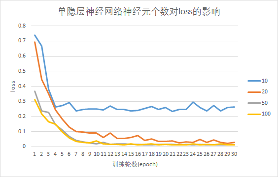
可见随着训练轮数增长,各个模型的训练集loss首先快速下降,接着缓慢下降。单隐藏层神经元个数越多,训练完成后的loss越低,说明增加神经元宽度能提升模型对目标函数的拟合能力。

增加隐藏层深度对拟合效果的影响

考察神经网络分别包含1、2、3、4个隐藏层,且每个隐藏层包含20个神经元时,训练集loss随训练轮数增加的变化情况(如下图)。(设置学习率为恒定值0.001,训练轮数为30轮)。

image-20201129232317776

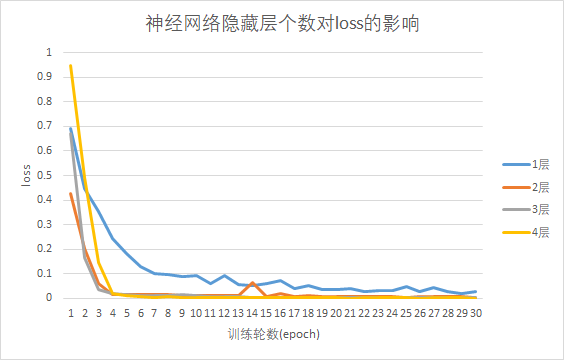
由图可见,神经网络层数越多,30轮训练结束后训练集的loss越低,说明层数越多,模型对目标函数的拟合能力越强。

最终效果

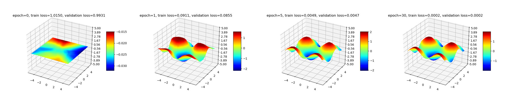
经过以上实验,我们验证了增加隐藏层的宽度和深度能减小拟合的误差。最后为了让拟合误差尽量小,经过多次尝试后,我们最终选择设置隐藏层个数为5,分别包含100、80、50、30、10个神经元,学习率衰减方案为每经过3轮训练,lr衰减为0.9倍。最终训练集loss为0.00015,验证集loss为0.00016。第0轮(训练前)、第1轮、第5轮、第30轮训练后的拟合结果可视化后如下图所示:

图片1

动图效果:

2

完整代码见:https://github.com/rubychen0611/MyNeuralNetwork